Spreadsheet tips for grading
Various spreadsheets have some lesser known formulas or functions that teachers can use for grading. I use these myself, and for the more complex ones, at the end of each semester as I calculate grades, I find myself having to look online again for instructions on some of these. So for my sake, and for other teachers, I have created this guide to help you. These should work for any spreadsheet program, but when necessary, subtle syntax differences between major spreadsheets, namely, Excel, Google Sheets, and LibreOffice Calc are mentioned.
Contents
1 Highlight alternating lines
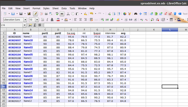
The first thing you may want to do is to highlight alternating rows so you can see the data more clearly. This can easily be done with conditional formatting in different spreadsheet programs.
- Excel
- Highlight the full range of cells in which you want alternating highlighting. From the Home tab, find and check the following options:
Home > Styles > Conditional Formatting > Manage Rules > New rule > Use a formula to determine which cells to format > Format values where this formula is true. Then enter this formula, and click Format:
- =MOD(ROW(),2)=1
In the Fill tab, select the color that you want to use for shading the rows.
- LibreOffice
- LibreOffice uses format styles for the word processor and for Calc, and a style with a colored fill pattern needs to be defined first, then it is applied to odd or even rows with conditional formatting. To define a style, create a new style from the menu bar (Format > Styles > New style) or from the style bar if it is open. For example, create a new style called "LineHilite". In the style properties box, right click on the style, and chose a color fill option on the fill tab. Then apply the style to alternating rows. From the menu bar, select the following: Format > Conditional Formatting > Condition. Change the leftmost tab from "cell value is" to "cell formula is", enter one of the following formulas, and chose the style to apply.
- ISEVEN(ROW()) - for even numbered rows
- ISODD(ROW()) - for odd numbered rows
- Google Sheets
- This program now has direct support for alternating line colors. Highlight all the cells in your sheet, and then from the menu bar, chose Format > Alternating colors. Chose the fill color that you want, and apply it. Before this feature appeared, the way to do it was Format > Conditional formatting > Format cells if > Cell formula is, enter an ISEVEN(ROW()) or ISODD(ROW()) formula, and chose the fill color.
For whichever program you use, the standard palette of fill colors may be too dark. You can define a custom color that is more eye-friendly. I chose the lightest gray available, and then click the custom color option. You can modify this choice in different ways, e.g., by using the color wheel and changing the darkness. I like the HTML color codes, which I am used to. The default light gray is, say, #f5f5f5, which I can change to to #f9f9fc for a very light blue-gray that is easier on my eyes.
2 Curving grades
Let's say you give a quiz that a lot of students did poorly on, but a few did okay. Out of fairness, you would like to curve up the grades. You could just add a few points in the spreadsheet, or multiply the raw score by a number like 1.05; but if a few students scored in the upper 90s, you might have scores over 100 - which is fine if you like giving extra credit. Otherwise, you will need to use a conditional formula to put an upper limit on the score. I will use mathematical functions with f(x) for the raw score, with examples of spreadsheet formulas.
f(x) = x+2  -> =B2+2  (additive)
f(x) = x*1.05 -> = 1.05*B2  (multiplicative)
You can use a conditional function ("IF") to make sure grades to not exceed 100.
=IF(condition, if-true, if-false)
The first statement in the parentheses states the condition, for example, if cell B2 with a score multiplied by 1.05 is less than 100, then the adjusted score is 1.05x; but if it would exceed 100, then simple assign a score of 100. You can use the less-than symbol (<), or "<=" for the less-than or equal-to symbol in spreadsheets.
=IF(1.05*B2<=100,1.05*B2,100)
If you are feeling stingy or grinchy, you can of course adjust grades down by subtracting or by multiplying with an integer below 1.0.
=B2-2 (subtractive)
=.98*B2 (multiplicative)
However, if a few students did well, but many did poorly, then an exponential curve can be done using a square root function. Students receive an increase proportional to how poor their score is. Those with high scores receive little or no increase, those with medium scores receive a greater boost, and those with low scores receive the greatest increase, proportionally. This can be the fairest option for a difficult test or assignment. This is done by taking the square root of the raw score and multiplying by 10.
f(x) = 10√x
This can be done easily in spreadsheets with the POWER function, or if you prefer a slightly more complicated way, the carat symbol (^) to raise a number to 0.5.
=10*(B2^.5)
=10*POWER(B2, 1/2)
If this leads to too much of an increase for you, you can do a moderate or adjusted square root curve, by averaging the square-adjusted score with the raw score, which curves the grades by half as much as the square root adjustment. The curve is still proportionally greater for lower scores, but the amount of increase overall is halved.
f(x) = (10√x + x) / 2
=AVERAGE(B2,(10*POWER(B2,1/2)))
The following table compares these methods for raw scores (x).
| raw score | simple curve | adj. simple curve | sq. root function | adj. sq. root function | curve down |
|---|---|---|---|---|---|
| x | 1.05x | 1.05x if x≤100 | f(x) = 10√x | f(x) = (10√x + x) | .98x |
| B2, B3, ... | =1.05*B2 | =IF(1.05*B2<=100,1.05*B2,100) | =10*POWER(B2, 1/2) | =AVERAGE(B2,(10*POWER(B2,1/2))) | =.98*B2 |
| 100 | 105.0 | 100.0 | 100.0 | 100.0 | 98.0 |
| 99 | 104.0 | 100.0 | 99.5 | 99.2 | 97.0 |
| 97 | 101.9 | 100.0 | 98.5 | 97.7 | 95.1 |
| 95 | 99.8 | 99.8 | 97.5 | 96.2 | 93.1 |
| 92 | 96.6 | 96.6 | 95.9 | 94.0 | 90.2 |
| 90 | 94.5 | 94.5 | 94.9 | 92.4 | 88.2 |
| 89 | 93.5 | 93.5 | 94.3 | 91.7 | 87.2 |
| 88 | 92.4 | 92.4 | 93.8 | 90.9 | 86.2 |
| 85 | 89.3 | 89.3 | 92.2 | 88.6 | 83.3 |
| 81 | 85.1 | 85.1 | 90.0 | 85.5 | 79.4 |
| 78 | 81.9 | 81.9 | 88.3 | 83.2 | 76.4 |
| 75 | 78.8 | 78.8 | 86.6 | 80.8 | 73.5 |
| 70 | 73.5 | 73.5 | 83.7 | 76.8 | 68.6 |
| 64 | 67.2 | 67.2 | 80.0 | 72.0 | 62.7 |
| 0 | 0 | 0 | 0 | 0 | 0 |
3 Dropping the lowest score
For a set of homework assignments, you want to drop the lowest score for calculating students' homework averages. The easiest way to drop one low score is to use the MIN function to find the lowest number in a range and remove it from the range of numbers to be summed and average. For these score-drop functions, the SUM/n function (n=number of scores) works better than the AVERAGE function. The MIN function requires a range, that is, the cells with one student's scores.
=MIN(range)
=MIN(A2:L2)
This finds the lowest score, and this function can be plugged into the SUM function to remove the lowest score and average the remaining scores.
=(SUM(A2:L2)-MIN(A2:L2))/10
Dropping more than one score requires the SMALL function instead, as MIN can only identify the very lowest score in a range. The SMALL function requires a range of cells, and the xth smallest number that you want, e.g., the very smallest (1), the second smallest (2), the third smallest (3), and so on.
=SMALL(range, xth-smallest)
=SMALL(A2:L2,1)
=SMALL(A2:L2,2)
These can be plugged into the summation formula, and you can use either MIN or SMALL(range,1) to identify the lowest score. Either of these formulas will average a students' scores minus the lowest two.
=SUM((A2:L2)-MIN(A2:L2,1)-SMALL(A2:L2,2)/10
=SUM((A2:L2)-SMALL(A2:L2,1)-SMALL(A2:L2,2))/10
4 Counting instances
The COUNTIF function can count the number of times that an item occurs in a range of cells. For example, I track students' absences and tardies in a spreadsheet. At the end of the semester, I tally them to deduct points from their participation grades. The COUNTIF function requires a range of cells to evaluate, and the target item that you are looking for. If it is in text format, enclose it in quotation marks, and if it is a range of numbers, make sure that the cell text format is text or numeric, as this might affect how these and other functions work (highlight the cells and press CTL-1 to check the cell format).
=COUNTIF(range, "target")
For example, I want to count the number of tardies for student A, marked "l" for late, and the number of unexcused absences, marked "x" in my spreadsheet.
=COUNTIF(A2:AA2,"l")
=COUNTIF(A2:AA2,"x")
4.1 Two conditions, e.g., count between two values
The COUNTIFS function allows you to specify two conditions. You can specify two conditions over two different ranges, or you can enter the same range twice if you want to count something between two values.
=COUNTIFS(range1, condition1, range2, condition2)
In this example, I want to count the number of final averages in the B range.
=COUNTIFS(T2,"<90",T2,">=80")
In this example, I want to count the number of A grades for students whose major is identified as engineering in column C that lists their majors.
=COUNTIFS(T2,"<=90",C2,"Engineering")
4.2 Counting multiple values in a range
The COUNTIF function may not work if the target value is a value from another cell (A2, B2, C2...), i.e., to count the number of occurrences of a number of values. In this example, I have all my students' ID numbers, and I want to search for how many times they submitted an online form (using their ID numbers). There are many target values, and a range to search for in another sheet or tab. A more complicated formula may be necessary if COUNTIF does not work.
=SUMPRODUCT((LEN(range)-LEN(SUBSTITUTE(range,value,"")))/LEN(value))
So here I've got a range in another sheet called 'Form responses 1', and I have a column to the left of the formula with all the student ID numbers (A2...). I want to count how many times each student submitted a form and thus, how often each ID number occurs in the range (they entered their ID each time they submitted the form, which Google Forms put into a spreadsheet). So I will enter this formula in the first cell and drag it down with the mouse to the other cells. Because I want the range to stay the same, I used dollar signs for cells in the range to specify an absolute range.
=SUMPRODUCT((LEN('Form responses 1'!$C$2:$C$134)-LEN(SUBSTITUTE('Form responses 1'!$C$2:$C$134,A2,"")))/LEN(A2))
5 Conditional function
The conditional IF function, as seen above, evaluates a condition on a target cell or cell range, and enters data in the current cell according to whether the condition holds true for the cell(s), and what to enter if not.
=IF(condition, if-true, if-false)
The condition itself can be a simple equation with an equality (=), inequality (< or >), greater than or equals (=>) or less than or equals (<=). If an element in the condition is a text string, quotation marks are used, and usually quotation marks are needed for the if-true and if-false statements. For example, if a neighboring cell contains an "x", a 0 is entered in the current cell, but if not, then a 1 is entered.
=IF(A2="x",0,1)
Other examples:
=IF(A2<100,"yes","no")
=IF(A2<=100,"yes","no")
This formula evaluates cell A2, takes the score from cell B2, adds or deducts one point from B2 depending on the value of A2, and enters it into the current cell.
=IF(B2="x",A2-1,A2+1)
Conditional statements can be plugged into larger formulas. For example, I assign a basic participation grade for in-class participation, but I deduct points for more than two absences, that is, if the number of absences (reported in cell X2, from the previous COUNTIF function) exceeds 2.
=Z2-(IF(X2>2,(3*(X2-2)),0))
This can be broken down like so:
condition: IF(X2>2)
then: Z2 - (3*(X-2)
else: Z2 - 0
altogether: =Basic participation in Z2 - [IF X2 > 2, then (3-point-penalty)*(#absences -2)]
To make things more complicated, the COUNTIF function could be embedded into the above conditional, which evaluates the attendance list (cells 2 to T2 for this student) and deducts points all in one complicated function. The more complicated a formula becomes, the easier it is to make syntax errors, e.g., with opening and closing parentheses.
=IF((COUNTIF(C2:T2,"x")>2),Z2-(3*(X2-2)),Z2)
6 Combining data across tabs or sheets
Sometimes data in one set of columns, or on separate sheets or tabs of a spreadsheet file, need to be merged together - or even between separate files. This is more difficult when the data are not sorted or ordered in the same way, so that you cannot just copy and paste columns from one sheet into the other. This is not too hard to do, and does not require any extra third-party extensions or apps beside the basic spreadsheet, but it does involve a more complicated function with syntax that is less intuitive (and not explained so clearly on some websites).
For example, I have a spreadsheet with two sheets for each class section - one for the students' attendance roster, and one for their grades. The attendance list is sorted alphabetically by student names, so I can print it out, easily check attendance, and enter the data in the spreadsheet. But the grade list is sorted by student ID number, because that is how I have to enter the grades in my university's computer system. So I have to merge attendance and participation data and grades into the grade sheet.
For this, we will use the VLOOKUP function (i.e., vertical lookup), which looks up data from one range vertically (row by row, based on an identifier) and merges it into a second data range that is sorted differently. The syntax requires the following (using my own terminology for clarity). I will refer to the range from which you want to take data as the Source, and the sheet into which you want to merge it as the Target (the sheet in which you are working and into which you are inputting the data via VLOOKUP).
=VLOOKUP(Identifier, Source-range, Column#, Approx.-value)
- Identifier: A reference variable that appears in both data ranges, which you will use to identify the students in each range. (In my example, this is the student ID number.) In the formula, I identify this unique Identifier according to the column number in the Target sheet, e.g., if ID numbers are in column B2 in the Target sheet, that is the identifier in the VLOOKUP formula.
- Source-range: The range of rows and columns in the Source-range that you want to consider, from the Identifier all the way to the column you want to import. The Identifier column should be the leftmost column in the Source range. The formula matches the above Identifier with the leftmost column of the Source-range. The Source-range will include the tab name plus a range of rows and columns.
- Column-number: The xth column from the identifier, which you want to take and input into the Target sheet. In other words, the column number with the source data you want to import into the current (target) sheet. VLOOKUP does not want the column label or header, but it wants to know how many columns away from the Identifier it is, so this will always be a whole number (2 columns away, 50 columns, or such).
- Approximate-values - true / false? Is an approximate match of values okay - true or false? You would want exact matches for student names, IDs, or grades, so you should enter FALSE.
Your source and target data ranges might be in different parts of the same sheet, but more likely, they are in separate tabs in a spreadsheet file, or even in different files.
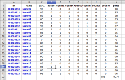
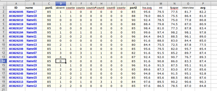
In my example below, Sheet1 contains the source data, i.e., the students' ID numbers, attendance information, and participation grades, which I want to merge into the target Sheet2, the grade data. I could use the Data Sort functions to rearrange rows and copy the data to the other sheet, but I want to continuously update both sheets with new grade and attendance information throughout the semester. (My participation/attendance sheet is in alphabetical order, which is convenient for checking attendance, but the final data need to be ordered by student ID number for turning grades at my uni.) The best course is to use VLOOKUP formulas so they can continually update while keeping. As data are added to the source sheet, the target sheet data should automatically update. This also makes it easier to email students complete grade and attendance information (see below about email merging).
The unique Identifier in both tabs is the student ID number. I have to identify the whole Source range, with the Identifier being the leftmost column of this Source-range - in my case, it is the ID number in column A. Note that in this example, the Identifier is in row B in the target sheet, but row A in the Source-range. In the source range, I want to copy the number of absences in Source-range row AX, which is located 50 rows away from column A. Thus, the column number in the formula is 50. In row C of the Target sheet, I will enter the formula for the first student in row 2 like this. The dollar signs in the formula will preserve the correct Source-range as I drag and copy the formula down to the other rows.
=VLOOKUP(B2, 'Sheet1'!$A$2:$AX$11,50,FALSE)
Some comments.
- Dollar signs
- If you enter the formula in row 2 for Student A, and then drag it down with your mouse to fill the other rows, the values of the Source-range will change for each cell, because spreadsheet programs assume you want the values for each cell. We want to update the Identifier for each row (B2, B3, B4 ...). However, we want to use the very same Source-range for all the students in the target sheet. To prevent this, we use the syntax for what is called a data array, or a set of absolute cell references. This is done by putting a dollar sign before each letter and number in the cell range, making each row and column an absolute value.
Alternatively, in Excel you could enter the formula without dollar signs, and enter the VLOOKUP formula into the cell by pressing CTRL-SHIFT-ENTER instead of ENTER, and it will make them absolute values (curly braces will then appear around the array name). Another option is to first highlight the Source-range and manually give it a special array name (e.g., Data > Define range from the menu bar), and enter the array name in the formula, e.g., =VLOOKUP(B2,Attendance,50,FALSE).
- Sheet name
- For the Source-range, you have to give the sheet name (tab name) plus the data range in that sheet. The data range itself is a range of rows and columns, A2:AX11. The tab name is appended to the beginning in Excel with single quotes and an exclamation mark. Different programs may do this slightly differently; see below. Some programs like Excel allow you to import data from a different file, preferably in the same directory, with square brackets around the file name. Note that these syntax details may change between programs and program updates.
- Excel: 'Sheet1'!$A$2:$Z$30
- LibreOffice 5: 'Sheet1'.$A$2:$Z$30
- LibreOffice 6: $'Sheet1'.$A$2:$Z$30
- Google Sheets: Sheet1!$A$2:$Z$30
- Excel, import from a different file: [filename.xlsx]Sheet1!$A$2:$Z$30
After entering the VLOOKUP formula for the first student and making sure it works properly, we can drag it down with the mouse to copy it into the other rows. We can then go to the next column and enter another VLOOKUP formula to copy the participation grades from column AY in the Source sheet to the Target like so:
=VLOOKUP(B2, 'Tab1'!$A$2:$AX$11,51,FALSE)
The How-To Geek website has a useful explanation of VLOOKUP here. There is also a horizontal lookup function, HLOOKUP, which works similarly.
7 Text & number format problems
Sometimes you may find that a formula is not working properly, e.g., giving erroneous results, or displaying an error message. Often this is because the range of cells in question is in text format, when the function requires numerical format. This can be solved by highlighting the cells, pressing CTL-1, and changing the format from text or general to numeric.
You may find extraneous lead apostrophes in cells, for example, '10 instead of 10. This is particularly a problem in LibreOffice, either after converting cells from text to numeric format, or pasting in data from another program, or importing data from another file format like CSV. LibreOffice has a tool to correct this. Highlight the cells, and on the menu bar, find Data > Columns to text, and click OK to apply it to the cells. Problem solved.
8 Email merge
I like to email students feedback on major assignments or final grades. It is possible to do automated email merges with a spreadsheet. In Google Sheets / Docs, there are third-party apps or scripts that can be installed, but I find them rather clunky or complicated. Some like Doctopus are popular, but are really designed for other tasks, like collaborative student work on files or sharing files and giving feedback via text documents.
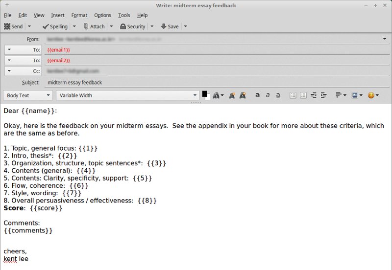
The easiest method that I have found is to use the free Thunderbird email client, and install the mail merge extension. I create a spreadsheet with grades and comments for each student, and the spreadsheet must be exported to a CSV file (comma separated values, a type of text file with commas separating each "cell" of data). Each column has a simple plain text header (e.g., student name, ID, comments, grade, email). (Note: the Thunderbird mail merge plugin seems to not like non-Latin text, like student names in Chinese or Korean text.)
In Thunderbird, I create a mail template (find 'Template' in the mailboxes for the email account), and compose a standard template. In the template, double square braces are used as placeholders for the row name from the CSV spreadsheet. After composing it, chose Send > Mail merge, and browse for the CSV file (you can leave the other options as they are). Click "send now" and watch it send a personalized email to each student with his/her feedback and grade information. More detailed instructions can be found here.
9 Links
- Thunderbird: A Firefox-based email client
- Thunderbird add-ons (extensions, such as mail merge utilities)
- LibreOffice: A free open-source office suite


